Solving Data-Constrained FEM Problems with Firedrake and stat-fem
Eric Daub, Research Engineering Group, Alan Turing Institute
(Theory due to Mark Girolami, Cambridge)
Talk given at the Firedrake ’21 Conference (Virtual), September 2021 and slightly modified to be a standalone part of documentation.
import numpy as np
from firedrake import UnitIntervalMesh, FunctionSpace, TrialFunction, TestFunction
from firedrake import SpatialCoordinate, dx, Function, DirichletBC, solve
from firedrake import dx, pi, sin
import matplotlib.pyplot as plt
from scipy.stats import multivariate_normal
from stat_fem.covariance_functions import sqexp
firedrake:WARNING Could not find BLAS library!
firedrake:WARNING OMP_NUM_THREADS is not set or is set to a value greater than 1, we suggest setting OMP_NUM_THREADS=1 to improve performance
Note: This cell was not part of the talk as it defined the mis-specified FEM that was solved as part of the example.
def measurement(measure_pts, error):
    assert error > 0.
    assert np.all(np.array(measure_pts) > 0.)
    assert np.all(np.array(measure_pts) < 1.)
    nx = 101

    mesh = UnitIntervalMesh(nx - 1)
    V = FunctionSpace(mesh, "CG", 1)

    u = TrialFunction(V)
    v = TestFunction(V)

    x = SpatialCoordinate(mesh)
    xp = Function(V)
    xp.interpolate(x[0])

    xvals = np.reshape(xp.vector().dat.data, (-1, 1))

    np.random.seed(24435)
    fvals = multivariate_normal.rvs(size=1,
                                    mean=np.pi*np.pi*np.sin(np.pi*xvals.flatten()),
                                    cov=sqexp(xvals, xvals, -1., -4.))

    f = Function(V, val=fvals)

    a = (u.dx(0)*v.dx(0) + u*v) * dx
    L = f*v*dx

    bc = DirichletBC(V, 0., "on_boundary")

    u1 = Function(V)

    solve(a == L, u1, bcs=[bc])

    return np.random.normal(size=len(measure_pts),
                            loc=u1.at(measure_pts),
                            scale=error)
Data and FEM models
How do we use data to inform/constrain FEM models in a manner that respects different types of uncertainties, does not overfit data, and is computationally efficient?
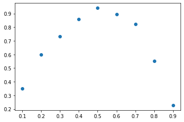
Simple example solving the time-independent heat equation in 1D. Imagine that we go into the laboratory and heat a 1D material and measure the resulting temperature. We might get something that looks like the following:
%matplotlib inline
import matplotlib.pyplot as plt

pts = [0.1*float(x) for x in range(1, 10)]
error = 5.e-2
data = measurement(pts, error)
plt.plot(pts, data, "o");
Firedrake solution
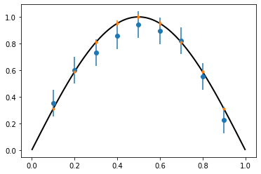
Straightforward to solve the underlying PDE using Firedrake on a unit interval mesh using piecewise-linear basis functions and compare with data (which we plot with error bars this time). Rather than returning the solution, I return the assembled linear system and function space used to construct the solution as I will need these later to carry out the statistical FEM solution.
from firedrake import UnitIntervalMesh, FunctionSpace, TrialFunction, TestFunction
from firedrake import SpatialCoordinate, Function, DirichletBC, assemble, solve
from firedrake import dx, pi, sin, plot

def generate_assembled_fem():

    nx = 101

    mesh = UnitIntervalMesh(nx - 1)
    V = FunctionSpace(mesh, "CG", 1)

    u = TrialFunction(V)
    v = TestFunction(V)

    x = SpatialCoordinate(mesh)
    f = Function(V)
    f.interpolate(pi*pi*sin(pi*x[0]))

    a = u.dx(0)*v.dx(0)*dx
    L = f*v*dx

    bc = DirichletBC(V, 0., "on_boundary")

    A = assemble(a, bcs=bc)
    b = assemble(L)

    return V, A, b
def plot_solution(u, pts, data, error):

    fig = plt.figure()
    ax = plt.axes()
    plt.errorbar(pts, data, yerr=error, fmt="o")
    plot(u, axes=ax)

V, A, b = generate_assembled_fem()
u = Function(V)
solve(A, u, b)
plot_solution(u, pts, data, 2.*error)
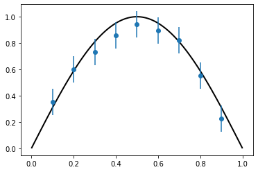
Model and data disagree
The model and the data are somewhat different – too many points lie far from the FEM solution. We know the uncertainty in the data, what about the model?
Could we have the wrong thermal conductivity?
Forcing of the heated material might be different than we guessed?
Are we solving the wrong equation?
How do we account for these in a principled way that respects uncertainties?
Add a fitting parameter
What people often do: RHS is probably uncertain, so we should just add a fitting parameter. This can be done in a straightforward manner using Maximum Likelihood Estimation.
def solve_heat_freeparam(coeff):

    assert coeff > 0.
    nx = 101

    mesh = UnitIntervalMesh(nx - 1)
    V = FunctionSpace(mesh, "CG", 1)

    u = TrialFunction(V)
    v = TestFunction(V)

    x = SpatialCoordinate(mesh)
    f = Function(V)
    f.interpolate(coeff*pi*pi*sin(pi*x[0]))

    a = u.dx(0)*v.dx(0)*dx
    L = f*v*dx

    bc = DirichletBC(V, 0., "on_boundary")

    u = Function(V)

    solve(a == L, u, bcs=[bc])

    return u
import numpy as np
from scipy.optimize import minimize

def mle_estimation(pts, data, error):

    def loglikelihood(coeff, pts, data, error):
        new_coeff = np.exp(coeff)[0]
        u = solve_heat_freeparam(new_coeff)
        soln = u.at(pts)
        return 0.5*np.sum((soln - data)**2/error**2)

    result = minimize(loglikelihood, 0., args=(pts, data, error))

    coeff = np.exp(result["x"][0])

    print("MLE result: {}".format(coeff))
    print("Number of FEM solves: {}".format(result['nfev']))

    u = solve_heat_freeparam(coeff)
    plot_solution(u, pts, data, 2.*error)
mle_estimation(pts, data, error)
MLE result: 0.9442305553763476
Number of FEM solves: 14
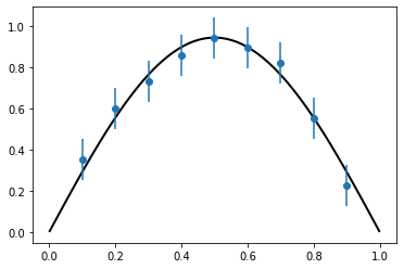
Are we any better off?
Maybe – the model fits the data better, but we added a free parameter. Were we justified in adding that free parameter? Does its value respect the uncertainties in the equation and the base physical system that we are studying?
A better approach is what follows, where we actually try to account for the uncertainty in our numerical model. I’ll look at the impliciations of an uncertain RHS of the governing equation, but we can equally do the same for the thermal conductivity.
FEM with uncertain RHS
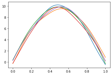
We can capture uncertainty information about the FEM by describing the RHS of our system as a Gaussian Process. A Gaussian Process is a distribution over functions with known mean and covariance:
Where \(f \sim \mathcal{GP}(\bar{f}(x), c(x, x))\). This is like a probability distribution, with the random variates being functions rather than variables. Draws from this distribution are functions that satisfy the mean and covariance properties. Covariance function \(c\) is assumed to be a squared exponential and depends on two parameters: a covariance scale \(\sigma_f^2\), and a correlation length \(l_f\).
GPs obey linear transformation rules, which means that if the RHS of a linear PDE \(\mathcal{D}u = \bar{f}\) is a GP, then we can transform the GP to get the solution:
Below we show several draws from a Gaussian Process with a mean given by the RHS of the FEM above. Discrete points drawn from a GP follow a multi-variate normal distribution, so we simply compute the discrete version of the mean function and covariance matrix to draw random variates from this discrete approximation of a GP.
from scipy.stats import multivariate_normal

xcoords = np.linspace(0., 1., 101)

sigma_f2 = 0.135
l_f = 0.135

mean = np.pi*np.pi*np.sin(np.pi*xcoords)
cov = sigma_f2*np.exp(-0.5*((xcoords[np.newaxis,:] - xcoords[:,np.newaxis])/l_f)**2)

vals = multivariate_normal.rvs(size=5, mean=mean, cov=cov)

plt.plot(xcoords, vals.T);
Statistical Finite Element Method
To solve this problem numerically, then, just need to assemble the FEM \(Ax=b\), the discrete version of the covariance matrix \(G\) and do some additional FEM solves of the stiffness matrix \(A\) to determine the uncertainty implications of the forcing uncertainty. The FEM solution is then
The stat-fem package implements this discrete covariance matrix as a
wrapper to a PETSc matrix, and carries out the solves via the
solve_prior function. (solve_prior is so-called because it does
not condition on the data. Eventually we will condition on the observed
data to determine the posterior.)
import stat_fem

G = stat_fem.ForcingCovariance(V, -1., -4.)

obs = stat_fem.ObsData(pts, data, error)

mean, cov = stat_fem.solve_prior(A, b, G, obs)

plt.figure()
ax = plt.axes()
plt.errorbar(pts, data, yerr=2.*error, fmt="o")
plt.errorbar(pts, mean, yerr=2.*np.sqrt(np.diag(cov)), fmt=".")
plot(u, axes=ax);
FEM models conditioned on data
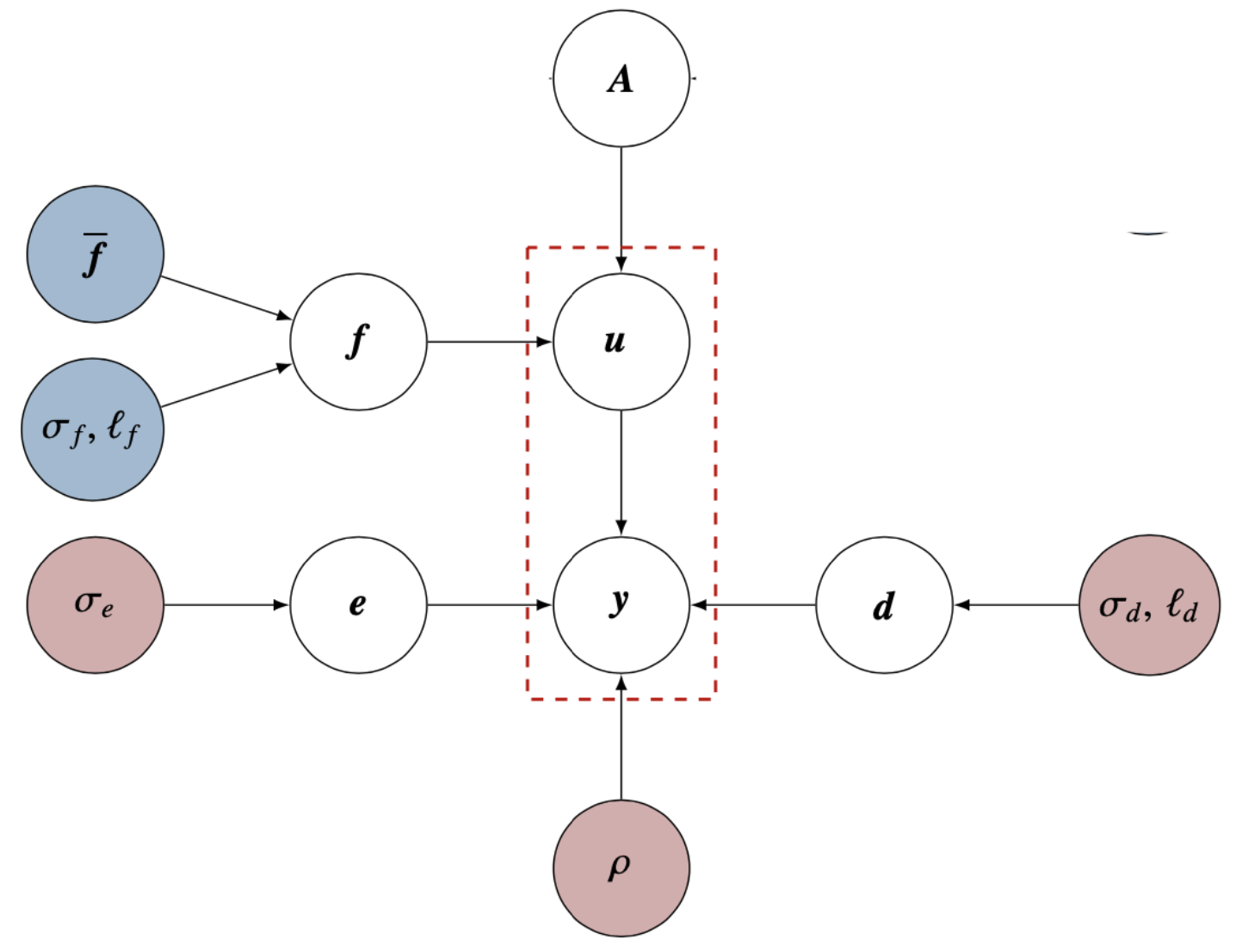
We now construct a framework where a heirarchical Bayesian model lets us perform statistical inference on data using FEM models.
Data is generated from \(y = \eta + e\), where \(\eta\) is the “true” physical process and \(e\) is statistical error due to measurement \(e \sim \mathcal{N}(0, \sigma_e^2 I)\).
\(\eta = \rho P u + d\) is then further decomposed into terms for the FEM solution and one that describes the discrepancy between model and reality.
The scaling factor \(\rho\) and model discrepancy \(d\) account for missing physics in the solution by explicitly separating this out from measurement error and known uncertainties in the governing equation.
\(P\) is an interpolation matrix that maps the FEM solution to the sensor locations.
\(d \sim \mathcal{N}(0, C_d)\), where \(C_d\) is the model discrepancy covariance, which accounts for spatial correlations in the model/data discrepancy (i.e. if the model is bad somewhere, it is probably bad for nearby points too). It depends on a covariance scale \(\sigma_d^2\) and correlation length \(l_d\).
FEM models conditioned on data
(Figure taken from [1])
[1] Mark Girolami, Eky Febrianto, Ge Yin, and Fehmi Cirak. The statistical finite element method (statFEM) for coherent synthesis of observation data and model predictions. Computer Methods in Applied Mechanics and Engineering, Volume 375, 2021, 113533, https://doi.org/10.1016/j.cma.2020.113533.
Estimation
Since all variables in the model are Gaussian (FEM solution u, model discrepancy, statistical error), then \(y\) is also Gaussian according to
We can use Maximum Likelihood Estimation to fit our model parameters \((\rho, \sigma_d, l_d)\). Requires 2 FEM solves per data point (the size of \(P\) is DOFx\(N_{data}\)) to compute \(\rho^2 P C_u P^T\), which only needs to be done once and can be cached.
Note that the MLE estimate finds a very small covariance, which indicates that there are no strong spatial correlations in the discrepancy between the model and the data, only an overall mean scaling correction. Thus, the correlation length parameter is not meaningful.
ls = stat_fem.estimate_params_MAP(A, b, G, obs)

# ls is a LinearSolver object with fit parameters

print("Model Discrepancy Fit:")
print("Scaling factor: {}".format(np.exp(ls.params[0])))
print("Covariance (sigma^2): {}".format(np.exp(2.*ls.params[1])))
print("Correlation length: {}".format(np.exp(ls.params[2])))
Model Discrepancy Fit:
Scaling factor: 0.9441016746283343
Covariance (sigma^2): 1.7150569288225287e-11
Correlation length: 9.438956152864298
FEM conditioned on data
From this model, we can estimate the parameters and compute the posterior \(p(u|y)\) – the posterior of the FEM model (this is implicitly conditioned on \((\rho, \sigma_d, l_d)\) as well, which are omitted for clarity, and will be estimated using MLE). Our prior beliefs are that the solution is \(u \sim \mathcal{N}(\bar{u}, C_u)\), and then our updated beliefs are that the mean is \(\bar{u}_{|y}\) and covariance is \(C_{u|y}\):
The mean is a weighted sum of the data and FEM, accounting for the various uncertainties in a principled way. The Covariance also balances the various sources of error.
In practice, don’t use above formulae directly, as \(C_{u|y}\) (DOFxDOF) is dense. Instead, use Woodbury Matrix Identity and compute \(P C_{u|y} P^T\) (i.e. compute the covariance only at locations where there are sensors) which requires \(2N_{data}\) FEM solves. (However, this still efficiently computes the mean for all DOF.) Then inference requires some additional inversion of dense \(N_{data}\)x\(N_{data}\) matrices and some matrix manipulations.
Note that the solution does not look very different from before – this is because once we respect all of the uncertainties (in particular the fact that the FEM solution is much more certain than the data measurements), the most likely explanation for the model-data discrepancy is some missing physics. We might expect there to be some change in the conditioned FEM solution if the reverse were true, and the data were more precise than the FEM solution.
u = Function(V)

ls.solve_posterior(u)

mean, cov = ls.solve_posterior_covariance()

plt.figure()
ax = plt.axes()
plt.errorbar(pts, data, yerr=2.*error, fmt="o")
plot(u, axes=ax)
plt.errorbar(pts, mean, yerr=2.*np.sqrt(np.diag(cov)), fmt=".");

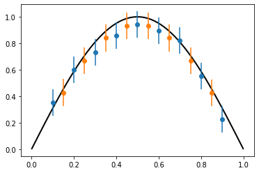
Predictive Distribution
Posterior predictive distribution \(p(y^*|y)\) is the posterior mean interpolated to the desired locations:
In practice, predicting the mean at some new location simply requires evaluating the mean at the new points. To compute the uncertainty, we need to do an additional 2 FEM solves for each prediction point to compute the covariance term.
new_pts = [0.1*float(x)+0.05 for x in range(1, 9)]

mean = ls.predict_mean(new_pts)
cov = ls.predict_covariance(new_pts, error)

plt.figure()
ax = plt.axes()
plt.errorbar(pts, data, yerr=2.*error, fmt="o")
plt.errorbar(new_pts, mean, yerr=2.*np.sqrt(np.diag(cov)), fmt="o")
plot(u, axes=ax);
Summary
Statistical FEM is a method for integrating data with FEM models in a Bayesian framework that accounts for uncertainties in a principled manner.
Rather than fit FEM directly to data, fit a heirarchical regression model to the difference through a model discrepancy. Tends to avoid problems of overfitting and regularization in direct fits while also making inference techniques more practical.
The method still makes robust predictions as the model can balance information from data with the physically-informed FEM solution and take uncertainties into account.
Straightforward to make predictions to test the model, with the long-term goal of this work being to build a “Digital Twin” that integrates a model with real-time sensor information from instrumented structures.
Comments on the Statistical FEM model
In most practical situations, we won’t actually be able to solve for the full covariance of the solution – computing the covariance of the solution requires 2 FEM solves per DOF, and will generate a dense matrix of size DOFxDOF. As shown above, we instead solve for the covariance at the data locations.
\(G\) is in reality a dense matrix, though if the correlation length of the covariance function are smaller than the domain size then in practice it can be approximated as sparse.
Unfortunately, can’t exploit this structure in advance, so the only way to form matrix remains to compute all elements and discard those below a threshold. Forming \(G\) thus remains a practical challenge for large problems.
Computing the covariance of the solution does parallelize well.
stat-femimplements it using Ensemble parallelism using Firedrake.