Poisson’s Equation Tutorial

This page provides an in-depth tutorial of the method applied to the solution of Poisson’s equation, a standard elliptic partial differential equation that is often used as an introduction to FEM problems. The tutorial illustrates how the equation would be solved in Firedrake, and then creates some synthetic data that is then used to condition the posterior solution to the FEM. Hyperparameter estimation is done using Maximum Likelihood Estimation.

The full Python script can be found in the file stat_fem/examples/poisson.py. We reproduce the relevant code here in the tutorial interspersed with the text.

Poisson’s Equation

Poisson’s Equation describes numerous phenomena, including heat diffusion, electrostatics, and the deformation of elastic bodies. It is commonly used as an example Elliptic Partial Differential Equation:

\[\nabla^2 u = -f\]

\(u\) here is the function that we wish to determine, which might represent the temperature in a 2D material. The function \(f\) is the external forcing, which is the local heat provided to the material at the given spatial location. The function is specified over the unit square, and the boundary conditions are assumed to be Dirichlet BCs, which set the values of the function at the boundaries (here assumed to be 0). We will assume that the function \(f\) has the form

\[f(x,y) = 8 \pi^2 \sin\left(2\pi x \right) \sin\left(2\pi y \right)\]

This has been conveniently chosen such that the analytical solution to the PDE is

\[u(x,y) = \sin\left(2\pi x \right)\sin\left(2\pi y\right)\]

which can be verified satisfies the BCs and the original governing Equation.

Solution with the Finite Element Method

To solve this problem using FEM, we must first convert to the weak form, which we do by multiplying by a test function \(v\) and integrate over the entire domain of interest \(\Omega\). We use the standard FEM procedure of integrating by parts to transform the Laplacian Operator \(\nabla^2\) into a dot product of gradients, and remove the surface integral term due to the boundary conditions:

\[\int_\Omega \nabla u \cdot \nabla v \; dxdy = \int_\Omega fv \; dxdy\]

We also need to specify a mesh subdividing the unit square into the subdomains over which we will approximate the function. Here we will use a triangular mesh and piecewise linear functions.

To solve this problem using Firedrake, we can use the built-in UnitSquareMesh, write out the above mathematical expression for the FEM in the Unified Form Language, set the boundary conditions, assemble the FEM, and then solve the PDE.

import numpy as np
from firedrake import UnitSquareMesh, FunctionSpace, TrialFunction, TestFunction
from firedrake import SpatialCoordinate, dx, pi, sin, dot, grad, DirichletBC
from firedrake import assemble, Function, solve
import stat_fem
from stat_fem.covariance_functions import sqexp
try:
    import matplotlib.pyplot as plt
    makeplots = True
except ImportError:
    makeplots = False

# Set up base FEM, which solves Poisson's equation on a square mesh

nx = 101

mesh = UnitSquareMesh(nx - 1, nx - 1)
V = FunctionSpace(mesh, "CG", 1)

u = TrialFunction(V)
v = TestFunction(V)

f = Function(V)
x = SpatialCoordinate(mesh)
f.interpolate((8*pi*pi)*sin(x[0]*pi*2)*sin(x[1]*pi*2))

a = (dot(grad(v), grad(u))) * dx
L = f * v * dx

bc = DirichletBC(V, 0., "on_boundary")

A = assemble(a, bcs = bc)

b = assemble(L)

u = Function(V)

solve(A, u, b)

Under the hood, Firedrake uses this information to assemble the linear system that we need to solve by creating the sparse matrix A representing the bilinear operator and the RHS vector b representing the forcing. This is a fairly straightforward operation using Firedrake. Once we have the linear system, we can create a Firedrake Function to hold the solution and then call the solve function, which will use the PETSc library to solve the system. If any of this is not clear, please consult the Firedrake documentation and examples for more guidance.

Data-Conditioned Solution to Poisson’s Equation

We will now create some synthetic data that will not perfectly match our prior FEM solution, and use the Statistical FEM to compute the updated posterior solution. First we generate some data with known statistical errors

# Create some fake data that is systematically different from the FEM solution.
# note that all parameters are on a log scale, so we take the true values
# and take the logarithm

# forcing covariance parameters (taken to be known)
sigma_f = np.log(2.e-2)
l_f = np.log(0.354)

# model discrepancy parameters (need to be estimated)
rho = np.log(0.7)
sigma_eta = np.log(1.e-2)
l_eta = np.log(0.5)

# data statistical errors (taken to be known)
sigma_y = 2.e-3
datagrid = 6
ndata = datagrid**2

# create fake data on a grid
x_data = np.zeros((ndata, 2))
count = 0
for i in range(datagrid):
    for j in range(datagrid):
        x_data[count, 0] = float(i+1)/float(datagrid + 1)
        x_data[count, 1] = float(j+1)/float(datagrid + 1)
        count += 1

# fake data is the true FEM solution, scaled by the mismatch factor rho, with
# correlated errors added due to model/data discrepancy and uncorrelated measurement
# errors both added to the data
y = (np.exp(rho)*np.sin(2.*np.pi*x_data[:,0])*np.sin(2.*np.pi*x_data[:,1]) +
     np.random.multivariate_normal(mean = np.zeros(ndata), cov = sqexp(x_data, x_data, sigma_eta, l_eta)) +
     np.random.normal(scale = sigma_y, size = ndata))

Here, y is the fake data, which has some statistical errors associated with it, and also differs from the true solution via a multiplicative scaling factor rho and a specified covariance sigma_eta and a spatial correlation scale l_eta. We also have a covariance scale sigma_f and correlation length l_f that describes the imperfect knowledge we have about the forcing function \(f\).

To find the posterior FEM solution, we can use the stat-fem library. We have already created the stiffness matrix A and the RHS vector b when we assembled the FEM, but we also need to represent our uncertainty in the forcing with a ForcingCovariance object and a ObsData object.

# Begin stat-fem solution

# Compute and assemble forcing covariance matrix using known correlated errors in forcing

G = stat_fem.ForcingCovariance(V, sigma_f, l_f)
G.assemble()

# combine data into an observational data object using known locations, observations,
# and known statistical errors

obs_data = stat_fem.ObsData(x_data, y, sigma_y)

The ForcingCovariance object holds the Sparse Matrix that represents the covariance matrix of the forcing using the PETSc library, and the ObsData object holds the information on the data, including the values, the spatial location of the measurements, and the statistical errors associated with those measurements.

Before we can compute the posterior solution, we need to determine how well we expect the data to match the solution. This is known as Model Discrepancy, which might represent missing physics in the FEM model or some calibration factor needed to match the data to the FEM solution. In some cases, we might have some prior knowledge of how well we expect the FEM to reproduce reality, while in others we may just want to use the data to estimate the mismatch so that we can use our model to predict things. In this case, we will estimate the parameters directly, as we have synthetic data that we know does not perfectly match. stat-fem has a built-in function for this, which will take a stiffness matrix, RHS vector, forcing covariance matrix, and data, and returns a LinearSolver object that has its model discrepancy parameters fit using Maximum Likelihood Estimation:

# Use MLE (MAP with uninformative prior information) to estimate discrepancy parameters
# Should get a good estimate of these values for this example problem (if not, you
# were unlucky with random sampling!)

ls = stat_fem.estimate_params_MAP(A, b, G, obs_data)

print("MLE parameter estimates:")
print(ls.params)
print("Actual input parameters:")
print(np.array([rho, sigma_eta, l_eta]))

From there, we can compute the mean posterior solution and determine its covariance:

# Estimation function returns a re-usable LinearSolver object, which we can use to compute the
# posterior FEM solution conditioned on the data

# solve for posterior FEM solution conditioned on data

muy = Function(V)

# solve_posterior computes the full solution on the FEM grid using a Firedrake function
# the scale_mean option will ensure that the output is scaled to match
# the data rather than the FEM soltuion

ls.solve_posterior(muy, scale_mean=True)

# covariance can only be computed for a select number of locations as covariance is a dense matrix
# function returns the mean/covariance as numpy arrays, not Firedrake functions

muy2, Cuy = ls.solve_posterior_covariance()

The script also makes some plots if Matplotlib is installed. These are reproduced below to show the expected output of the calculations if all works as expected.

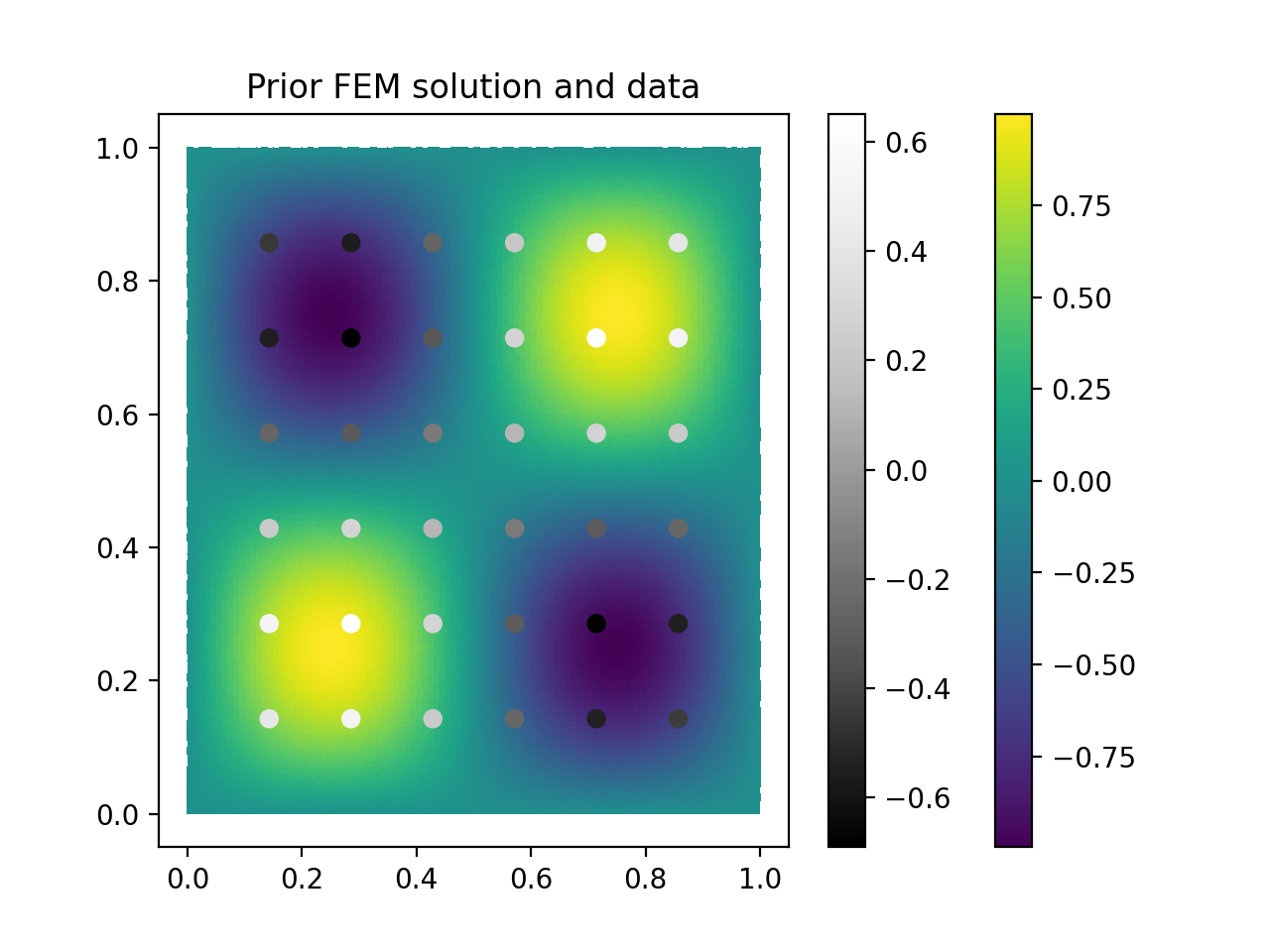
Prior FEM solution (color) and synthetic data points (greyscale circles) to the Poisson’s Equation problem. Note the mismatch between the color scales for the prior solution and the data.

Posterior FEM solution (color) and variance at data observation points (greyscale circles) to the Poisson’s Equation problem. Note that the color scale has changes, indicating that the posterior is now scaled to correctly match the data, and that the uncertainties are smallest close to the boundaries (where the solution values are most certain due to the known values at the boundaries), and largest at the center further away.